How to solve differential equations using convolutions
Suppose we have a function $u(x, y, t)$ that depends on space and time. Let’s say we want to describe a diffusion process. For example, $u$ could be the local temperature, or the concentration of a substance. The diffusion equation is:
\[\frac{\partial u}{\partial t} = \nabla^2 u\]For boundary conditions, we’ll assume that $u$ is zero at the edges of a square of side length $L$. Initially, we assume that $u$ is given by some function $u(x, y, 0) = f(x, y)$.
Analytical solution
We can solve this equation analytically using the method of separation of variables. I won’t go into too much detail, just the main idea.
We assume that $u(x, y, t) = X(x) Y(y) T(t)$ and substitute this into the diffusion equation:
\[X Y T' = X'' Y T + X Y'' T\]Dividing by $X Y T$ gives:
\[\frac{T'}{T} = \frac{X''}{X} + \frac{Y''}{Y}\]Each one of these terms depends on a different variable, so they must be equal to a constant. Let’s call this constant $-\lambda = -\mu^2 - \nu^2$. This gives 3 equations:
\[\begin{aligned} T' + \lambda T &= 0\\ X''/X + \mu^2 &= 0\\ Y''/Y + \nu^2 &= 0 \end{aligned}\]Note: the fact that the constants in 2nd and 3rd are positive can be derived from the boundary conditions.
The first equation will have a solution of exponential form: $T(t) = e^{-\lambda t}$. The second and third equations have an oscillatory solutions of the form $X(x) = \sin(\mu x)$ and $Y(y) = \sin(\nu y)$.
For given $\mu$ and $\nu$, the general solution is:
\[u(x, y, t) = A_{\mu, \nu} e^{-(\mu^2 + \nu^2) t} \sin(\mu x) \sin(\nu y)\]where $A_{\mu, \nu}$ is a constant.
The complete solution is a sum over all possible values of $\mu$ and $\nu$ compatible with the boundary and initial conditions.
To satisfy boundary conditions
\[u(x,0) = u(x,L) = u(0, y) = u(L, y) = 0\]we need to choose $\mu$ and $\nu$ such that $\mu = n \pi / L$ and $\nu = m \pi / L$ for integers $n$ and $m$.
And to satisfy the initial condition, we need to choose $A_{\mu, \nu}$ such that $u(x, y, 0)$ matches the series expansion of $f(x, y)$.
Numerical solution
Alternatively, we can solve this equation numerically. We’ll discretise space into a grid of $N$ points $(x_i, y_j)$, where $i$ and $j$ are integers (we can just refer to the points as $(i, j)$ to make it simple). We’ll also discretise time into a series of $M$ time steps $t_k$ up to a limit $t_M$.
The diffusion equation can be approximated by a “finite difference” equation. For a general function $f(x)$, the derivative $\partial f / \partial x$ can be approximated by the difference between the function at two nearby points:
\[f_+(x_i) = \frac{u(x_{i+1}) - u(x_i)}{\Delta x}\]where $\Delta x = L / N$ is the grid spacing. This is known as a “forward difference”. We can also have a “backward difference” which we’ll denote by $f_-(x_i)$:
\[f_-(x_i) = \frac{u(x_i) - u(x_{i-1})}{\Delta x}\]The second derivative can be approximated by a “central difference” where we take the finite difference of the forward difference and the backward difference:
\[\frac{\partial^2 f}{\partial x^2} \approx \frac{f_+(x_i) - f_-(x_i)}{\Delta x} \approx \frac{u(x_{i+1}) + u(x_{i-1}) - 2 u(x_i)}{\Delta x^2}\]The diffusion equation then becomes:
\[\frac{u_{i, j}^{k+1} - u_{i, j}^k}{\Delta t} = \frac{u_{i+1, j}^k + u_{i-1, j}^k + u_{i, j+1}^k + u_{i, j-1}^k - 4 u_{i, j}^k}{\Delta x^2}\]This equation can be rearranged as follows:
\[u_{i, j}^{k+1} = u_{i, j}^k + c (u_{i+1, j}^k + u_{i-1, j}^k + u_{i, j+1}^k + u_{i, j-1}^k - 4 u_{i, j}^k)\]with $c = \Delta t / \Delta x^2$.
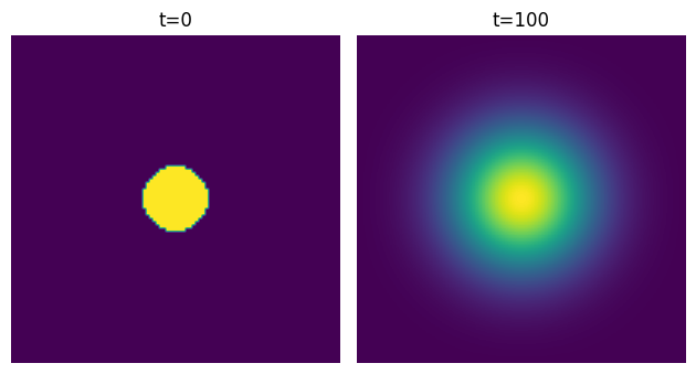
Here is some Python code that implements this algorithm (for simplicity we’ll use a small disk at the center as the initial condition):
import numpy as np

L = T = 100
N = 100
M = 1000
R = 10

dt = T / M
dx = L / N
c = dt / dx**2
x = np.linspace(0, L, N)
y = np.linspace(0, L, N)


def disk(x, y):
    return np.sqrt((x - L / 2) ** 2 + (y - L / 2) ** 2) < R

def solve_diffusion(u):
    for k in range(M):
        u[1:-1, 1:-1] += c * (
            u[2:, 1:-1] + u[:-2, 1:-1] + u[1:-1, 2:] + u[1:-1, :-2] - 4 * u[1:-1, 1:-1]
        )
    return u

u = np.zeros((N, N))
for i in range(N):
    for j in range(N):
        u[i, j] = disk(x[i], y[j])


u = solve_diffusion(u)
We can clearly see diffusion happening:
Convolutions
There’s a nice way to think about this problem as applying successive convolution filters to the initial condition, like how it’s done in image processing. The “image” in question is the initial condition, and the filter is this 3x3 matrix:
\[\begin{pmatrix} 0 & c & 0\\ c & 1-4c & c\\ 0 & c & 0 \end{pmatrix}\]from scipy import signal
def solve_diffusion2(u):
filter = np.array([[0, c, 0], [c, 1 - 4 * c, c], [0, c, 0]])
for k in range(M):
u = signal.convolve2d(u, filter, mode="same")
return u
We can show that these two functions are entirely equivalent, and indeed we get the same result.
Convolutions are widely used in image processing and machine learning, so there are various efficient implementations.
Now let’s see what happens when we try this with different initial conditions. Let’s place the disk lower, near the bottom edge of the square. The solution looks like this:
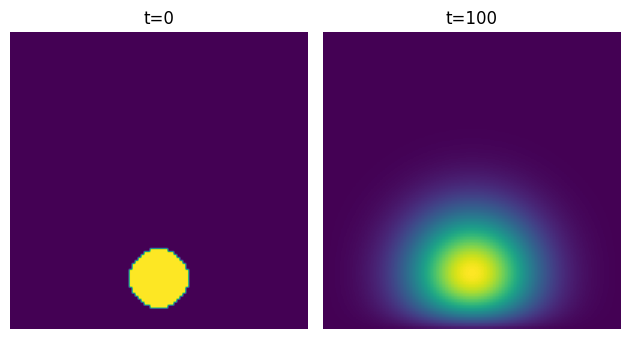
We can see something interesting happening there near the edge.
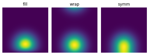
signal.convolve2d has a boundary argument that lets us specify what happens at the edges.
By default, it assumes that the image is surrounded by zeros - this is equivalent to our assumption that $u$ is zero at the edges.
Boundary conditions
Typically, we’d write the finite difference problem as a matrix equation and incorporate the boundary conditions into the matrix. This can be done by “flattening” the grid into a 1D array, writing the equation as $u^{k+1} = A u^k$ and carefully choosing the values for A.
Instead of doing that, we can look into how signal.convolve2d handles boundary conditions to get some inspiration.
The scipy implementation of signal.convolve2d is a wrapper around the C implementation which can be found here.
For the default argument fill, when the filter is applied at the edges of the image, any points outside the image are assumed to be zero.
This is equivalent to our assumption that $u$ is zero at the edges (to be precise, it’s equivalent to adding a 0 padding around the image).
The other options are wrap and symm.
wrap is equivalent to periodic boundary conditions: it pads the image with copies of itself.
symm, on the other hand, is equivalent to reflecting the image at the edges.
You can see the difference in the images below:
In the case where we are modeling the diffusion of a substance through a constrained volume, like a closed container, the appropriate boundary conditions are no flux conditions, also known as Neumann boundary conditions:
\[\frac{\partial u}{\partial x} = \frac{\partial u}{\partial y} = 0\]Incidentally, I always thought that they were called “von Neumann” boundary conditions, but they’re not.
In finite difference form, this becomes:
\[\frac{u_{i+1, j} - u_{i, j}}{\Delta x} = \frac{u_{i, j+1} - u_{i, j}}{\Delta y} = 0\]or
\[u_{i+1, j} = u_{i, j}\] \[u_{i, j+1} = u_{i, j}\]This is equivalent to reflecting the image at the edges, which is what symm does.
Non-rectangular domains
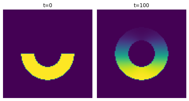
This methods gets a bit more complicated when we want to solve the diffusion equation on a non-rectangular domain. For example, we might want to solve it on a test tube or Petri dish.
We’ll assume that we have the cross section of a cylinder, and half of it is filled with a substance.
A naive application of signal.convolve2d wouldn’t do the job because our boundary conditions are not defined at the edge of the image.
We can try to apply the filter and then crop the result to the domain:
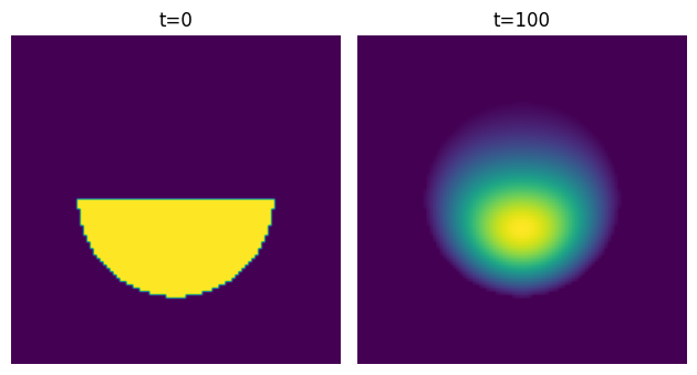
This looks quite nice, but it’s not correct. It’s essentially assuming that the concentration of the substance is zero near the edges, which is false.
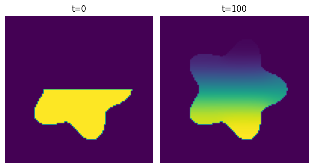
To fix this, we’ll first reflect the values at the edges of the domain - that enforces the right boundary conditions. Then we’ll apply the filter. Finally, we’ll set all the values outside the domain to zero and repeat the process.
To reflect the values at the edges, we can set the value of each point on the edge to the value of the nearest point inside the domain:
def find_edges(domain):
    kernel = np.array([[0, 1, 0], [1, 0, 1], [0, 1, 0]])
    boundaries = signal.convolve2d(domain, kernel, mode="same")
    return (boundaries > 0) & (domain == 0)


def reflect_at_edges(u, domain):
    edges = find_edges(domain)
    directions = [(1, 0), (-1, 0), (0, 1), (0, -1)]
    reflected_u = u.copy()

    for d_row, d_col in directions:
        shifted_domain = np.roll(domain, shift=(d_row, d_col), axis=(0, 1)).astype(bool)
        shifted_u = np.roll(u, shift=(d_row, d_col), axis=(0, 1))
        mask = edges & shifted_domain
        reflected_u[mask] = shifted_u[mask]

    return reflected_u
This is what the diffusion function looks like:
def solve_diffusion3(u, domain):
    filter = np.array([[0, c, 0], [c, 1 - 4 * c, c], [0, c, 0]])
    for k in range(M):
        u = reflect_at_edges(u, domain)
        u = signal.convolve2d(u, filter, mode="same")
        u = np.where(domain, u, 0)

    return u
This gives the correct result:
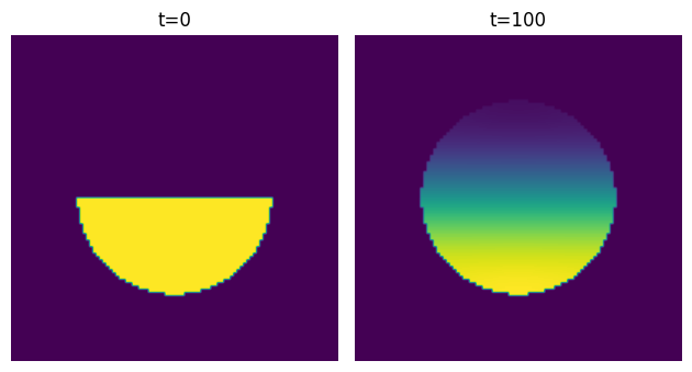
The cool thing about this is that it works for any domain - it doesn’t have to be symmetric:
Thanks to Thiago T. Varella for helpful suggestions