Climate change from first principles
One of the most urgent things that humanity has to do, we are told, is solving the climate crisis. Every 6-7 years the Intergovernmental Panel on Climate Change (IPCC) publishes an Assessment Report with a review of all published literature on climate change. That’s the most important authority on climate science. The 6th report (AR6) was published in 2021 and I gave a read to the Working Group I (WGI) contribution (Physical Science Basis).
I want to understand the basics of the models used to forecast climate change, what the most important findings are, what it means for humans and what can we do about it.
Disclaimer: I’m a mere software developer with a background in physics.
The Energy Balance model
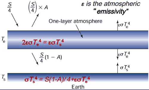
Schematic of one-layer atmosphere with the energy fluxes involved. Source
We start with a simple model where the Earth is considered a spherical black body with radius r.
In addition, we consider a single atmospheric layer around the Earth.
The incoming solar energy hitting the earth is
S = σ * T_sun ^4 * (R_s / D_SE)^2
where σ = 5.67 * 10^(-8) see the appendix for an explanation of there this formula comes from. R_s is the Sun’s surface radius and D_SE
is the Sun-Earth distance (this comes from energy conservation).
That energy gets spread over the Earth’s surface area 4 * π * r^2, so the incoming energy flux is
F = S * (1 - A) * (π * r^2) / (4 * π * r^2) = S * (1 - A) / 4
where A, the fraction of energy reflected by the atmosphere known as albedo, is typically taken as 0.3.
On the other hand, the outgoing energy from the earth is σ * T_E^4.
We can assume that a fraction ε of the outgoing radiation form the Earth is absorbed back by the atmosphere.
To be accurate, the atmosphere also absorbs a fraction of the incoming solar radiation before it makes it to the surface, but it’s a very small fraction that we can safely ignore.
With this model, using the Stefan-Boltzmann law, we can write the energy balance equation at each level: (1) atmosphere and (2) Earth’s surface. We get:
(1) ε * σ * T_E^4 = 2 * ε * σ * T_A^4
(2) F + ε * σ * T_A^4 = σ * T_E^4
where T_E is the Earth’s temperature and T_A is the atmosphere’s temperature. Solving this system of equations gives us:
T_E^4 = 2 * T_A^4
T_E^4 = S * (1 - A) / [4 * σ * (1 - ε/2)]
If we had a transparent atmosphere that absorbs none of Earth’s IR radiation (ε = 0),
we’d find T = 255 K, which is much colder than the 288 K average we have.
The reason for this is the greenhouse effect. This happens when e.g. CO2 molecules absorb this IR radiation and re-emit it, giving an ε ~ 0.77 and T = 288 K.
It’s worth noting that water is a much stronger greenhouse gas than CO2. However, CO2 happens to absorb radiation precisely at some of the wavelengths that water is transparent to and would normally take energy away from Earth.
So in simple terms, the earth is warming because too much energy is being reflected back by greenhouse gases. One of the immediate things that would keep Earth’s temperature low would be to increase the albedo A. This can be done by increasing Earth’s reflectivity and is called solar geoengineering.
But this model is oversimplified, for once it doesn’t consider that a lot of the energy flow in the atmosphere is due to evaporation (convection) and not irradiation. These kinds of complications, in addition to making this a 3-dimensional inhomogeneous model of Earth and the network effects that I’ll comment below, are the things that go into the most advanced climate models we have.
Climate Forcing Factors
Changes in the atmosphere (e.g. increases in the amount of CO2) translate into changes to the effective emissivity ε and albedo.
This introduces a complex network of interactions between the various components that affect the atmosphere.
For example, an increase in CO2 will increase ε, but with a higher temperature we will also have more H2O in the atmosphere,
and since water is itself a greenhouse gas, it leads to even more warming (positive feedback).
However, this extra water can form clouds, which increase the albedo, decreasing the warming (negative feedback). Water can have both warming and a cooling effect! That depends a lot on where these clouds are, what kind of clouds they are, etc.
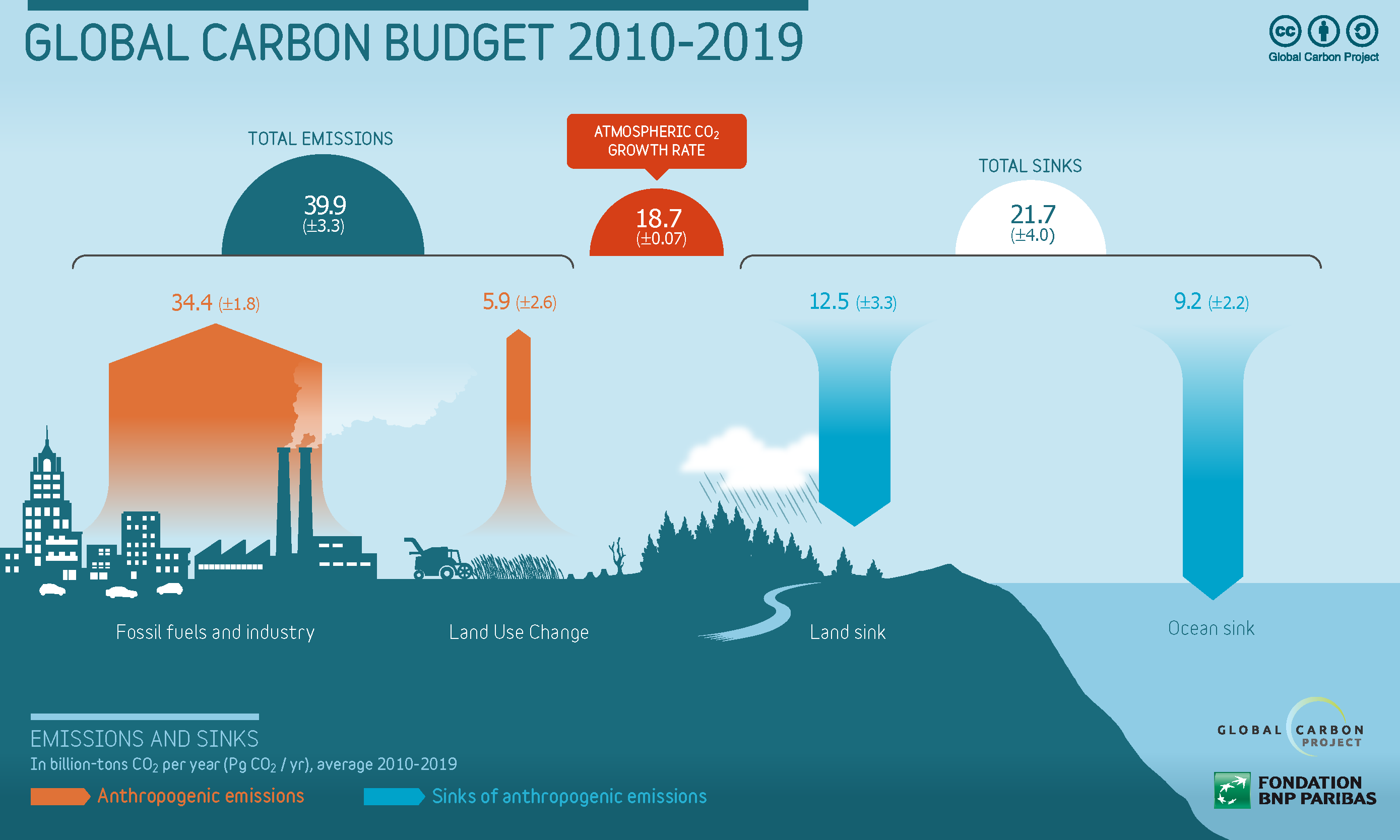
Another component is ocean chemistry. More CO2 in the atmosphere makes oceans more acidic, and that makes them worse CO2 absorbers. Biology is another factor. Plants and ocean algae absorb and release CO2 (through respiration and decay), but over a year, they are a net sink.
Estimates report that land and oceans absorbs around 22 GTon CO2 each year whereas human emissions have been on average around 40 GTon/year since 2010.
Another source of greenhouse effect is methane. It has a larger warming potential than CO2 - it has higher emissivity. If permafrost (frozen soil in the Northern Hemisphere with large amounts of biomass) begins thawing, lots of methane is going to be released into the atmosphere.
Finally, climate change is local. If air is humid (in tropics, lowlands, in summer) the greenhouse effect of water vapour overwhelms any effect due to CO2. In dry air, however - such as in the arctic, mountains, winter, at night - CO2 has a much stronger effect. So climate change makes cold places warmer much more than it makes hot places hotter.
Climate Sensitivity to CO2
To estimate climate sensitivity to various factors, we can ask:
if the energy imbalance F = outgoing_energy - incoming_energy increased to F + dF,
what would be the corresponding increase in temperature? We apply this to the Earth’s surface (from (2)):
F = σ * T^4 - S * (1 - A) / 4
(3) dF = 4 * σ * T^3 * dT
dF is called radiative forcing (W / m^2). It represents an out-of-equilibrium “force” that will end up changing the global temperature.
What dF can be expected from an increase in atmospheric CO2 concentration?
We empirically have that, for initial and final CO2 concentrations C_0 and C:
(4) dF = 5.35 (W / m^2) ln(C/C_0)
The reason for this logarithmic dependence has to do with the CO2 emission bands becoming saturated. Another reason is that the more CO2 we add, the height in the atmosphere at which those emissions happen will increase, and with increased height the temperature decreases, which from Stefan-Boltzmann law means less radiation. In other words, more CO2 has diminishing “returns” in the sense of radiation.
Plugging this into (3) with T=288K, we find that a doubling in CO2 concentration would mean a temperature increase of 0.68 K, which is not too far from what we observe right now (0.99 [0.84-1.10] K). Note however that this model disregards the feedback effects discussed above.
The IPCC projects that a CO2 concentration doubling would lead to a 3 [2.5-4] K temperature increase. That means that (4) would have to be multiplied by a factor of 4 [3.6-5.8] to account for the feedback effects.
Human Influence
According to the AR6:
It is unequivocal that human influence has warmed the atmosphere, ocean and land.
The sources of radiative forcing are: solar activity, volcanic activity (volcanic aerosols increase the Earth’s reflectivity and lower the temperature) and greenhouse gases.
Now, solar activity hasn’t changed much for thousands of years, nor has volcanic activity. It’s indisputable that atmospheric concentrations of CO2 have increased from 278ppm in the 19th century to 410ppm in 2019, which is a rate of growth unseen in the preceding centuries:
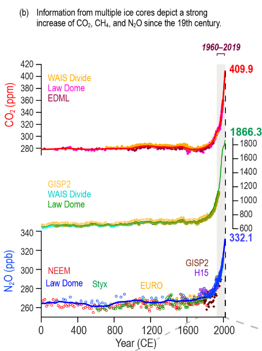
CO2 and N2O concentration evolution in time. Source: AR6
Our best simulations cannot reproduce the observed temperature increase without including human sources of radiative forcing:
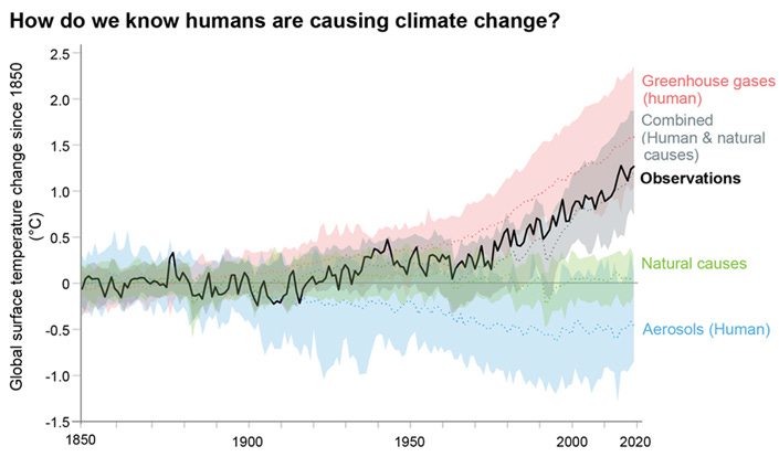
Average temperature change model prediction. Source: AR6
How do we know that humans are to blame for this increase? Aren’t there non-human processes that emit those gases into the atmosphere? Fossil fuels emissions from human activity account for ~85% of that 40 GtonCO2/year figure above (see section Climate Forcing Factors). They are the only source of carbon on Earth that could cause such a drastic increase in atmospheric CO2.
Another important piece of evidence is isotopes: we observe a decrease in C13 and C14 since 1990, which suggests that the rise in CO2 comes largely from fossil fuels which have low C13 and no C14.
Forecast
To improve climate sensitivity estimates, the IPCC puts together the predictions of climate models in the Coupled Model Intercomparison Project Phase 6 (CMIP6) of the World Climate Research Programme. These models tend to do very well: on historical data, their average temperature change is accurate within 0.2K.
The scenarios coming from CMIP6 range from an almost certain temperature increase of 1.5K (SSP1-1.9) until 2100, going up to 4-6K in the worst case (SSP5-8.5). These increases are reported in comparison to the period 1850-1900. In 2022 we were at about 1K.
‘SSPx’ refers to the Shared Socioeconomic Pathway describing the socioeconomic trends underlying the scenario,
and ‘y’ refers to the approximate level of radiative forcing (in units of W m–2) resulting from the scenario in the year 2100.
All scenarios predict 1.5K increase until 2040.
The report draws attention to the “arctic amplification effect”: high latitudes in the Northern Hemisphere warm up by 2-4x the average warming. This happens partly due to the loss of reflective sea ice. In the Southern hemisphere, ocean absorption makes the warming effect milder than global average.
In high latitudes of both the Northern and the Southern Hemisphere, precipitation will increase with the level of warming. The same happens for the tropics and the monsoon regions. Drying can be expected in subtropical regions - southern Africa and the Mediterranean will become progressively drier and warmer.
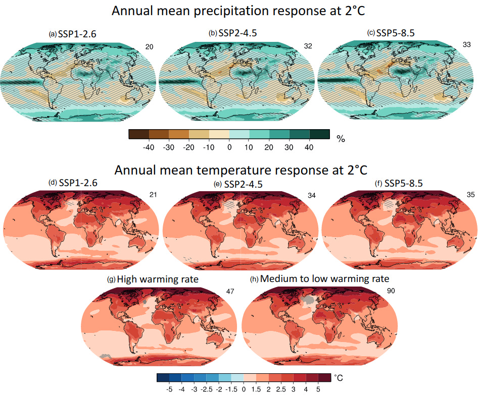
Local precipitation and temperature changes, averaged over all CMIP6 models (the number on the top right of each figure is how many models were averaged). There are indicated regions where the models don’t provide a very strong signal (diagonal lines) or where more than 20% of the models provide conflicting signals. Changes are relative to 19th century. Source: AR6
Due to ocean warming and ice sheet melting, sea levels are predicted to increase by 0.28-0.55m (SSP1-1.9) or 0.63-1.01m (SSP5-8.5) by 2100. However, it’s hard to say whether this is due to human causes.
One major concern is that an increase of ~2K would trigger a large number of tipping points in the climate system. These are thresholds that, when exceeded, cause more positive feedback loops to come into effect and accelerate the warming. That’s why the IPCC target is to keep climate change below 1.5K from pre-industrial levels (which was the goal of the Paris Agreement of 2015).
Carbon Budget
What is our carbon budget if we want to keep below the 2K target? For a very crude approximation we can correct formula (4) by a factor of 3.6 (in the best case scenario)to account for feedback loops (see section “Climate Sensitivity to CO2”):
ln(C/C_0) = 4 * σ * T^3 * dT / (5.35 * 3.6)
 = 4 * 5.67 * 10^(-8) * 288^3 * 2 / (5.35 * 3.6)
 = 0.56
With a starting concentration of 278 ppm (19th century), that is C = 488 ppm. Being currently at 412 ppm atmospheric CO2, that means we have left:
(488 ppm - 412 ppm) * (7.81 GtCO2 / ppm) ~ 593 GtCO2
with emissions of 40 GtCO2 per year, this gives us 14 years at the current rate!
In the worst case scenario, with a correction factor of 5.8, we would have already crossed the 2K threshold in terms of emissions, so that the only reason we haven’t seen that increase is because we’re not at the equilibrium point yet.
Impact
Whereas the WGI contribution has to do with science and modelling of the climate system, the Working Group II (WGII) contribution to AR6 is concerned with the impact that the forecasts above have to the environment and humans in particular.
According to WGII, climate change has already caused significant impact to ecosystems. As an example, we can take animal range patterns (that is, the area that an animal lives in during its lifetime). If we take all species living in areas where human land usage hasn’t changed for the past 20-250 years, about half of them have changed their range in directions consistent with what would be expected from warming trends - mainly poleward. (We look only at areas where land usage hasn’t changed because in areas where it has changed, land usage by humans is usually the main driver for species changing location.)
These changes have impacted humans too. One interesting example of this is the case of tropical diseases such as dengue, malaria and chukungunya occurring in non-endemic regions in Nepal - where the warming rate is higher than global average. (For many more examples see Table SM2.1 in AR6 WGII.)
According to the report, we can attribute to climate change the increased frequency and intensity of extreme heat and drought events - heatwaves, wildfires and floods, although it’s not possible to say which of the individual events can be directly related to human-induced climate change.
Curiously, climate change has caused both a decrease in agricultural productivity (in low latitude regions) and an increase (in high latitude). The extreme weather events have increased the risk of food insecurity in underdeveloped regions in Africa, Asia and America.
In the long term, we can expect these impacts to become more severe and for new effects to kick in, such as an increase in the risk presented by infectious diseases such as dengue.
When we try to forecast the socio-economic impacts of climate change, the climate factors interact so strongly with poverty and health that it’s hard to split one from another. The capacity to adapt to climate change will be strongly subject to the level of economic development of different societies. We can’t address one without addressing the other.
Conclusions
- Land + oceans absorb ~22 GTon CO2 each year whereas human emissions are around 40 GTon/year.
- Climate change makes cold places warmer much more than it makes hot places hotter.
- We might be near tipping points like permafrost thawing, but it’s really hard to tell.
- Atmospheric concentrations of CO2 have increased from 278ppm in the 19th century to 412ppm in 2019.
- This caused an unprecedented temperature increase (~1K from pre-industrial levels).
- We are sure that this increase was caused by greenhouse gas emissions from fossil fuels.
- The increase has been responsible for more frequent and extreme floods, wildfires and heat waves.
- Quote from AR6 Chapter 4:
it is only after a few decades of reducing CO2 emissions that we would clearly see global temperatures starting to stabilize. By contrast, short-term reductions in CO2 emissions, such as during the COVID-19 pandemic, do not have detectable effects on either CO2 concentration or global temperature. Only sustained emissions reductions over decades would have a widespread effect across the climate system
One of my takeaways from this is that it’s uncontroversial that human activity has increased the amount of CO2 in the atmosphere drastically, and that has resulted in an average temperature increase in the globe. But anything beyond that is very hard to predict at the moment: we don’t know what the effect of this human caused climate change will be on sea levels, hurricane activity and wildfires, if any. The increase in precipitation is one of the few exceptions where we are more certain on the impact.
In the worst case scenario, if we assume that human-driven climate change will have a major impact on earth, we will want to stop emissions immediately.
One of the best ways we can reduce fossil fuel emissions is using alternative energy sources like wind and solar, or a more reliable option like nuclear energy. It doesn’t emit greenhouse gases to operate, and the construction of nuclear facilities involves a relatively small amount of emissions.
We might need to seriously start removing CO2 from the atmosphere. But who will foot the bill? If we make oil companies pay for it, they will go bankrupt as their profit margins are already tight (low single digits). Government could pay for it, but right now it’s doing the exact opposite: subsidising oil so that transport and food is cheaper. Currently, escaping poverty creates unavoidable emissions, so it’s tricky for developed countries to ask developing countries to cut back. Our politician’s views on climate change should be one of the main factors in deciding how we vote.
References
This presents more detailed calculations.
IPCC AR6 Working Group I Report - especially the Summary for Policymakers, the Technical Summary and the FAQ in each of the chapters.
Appendix: the Stefan-Boltzmann law
This assumes some quantum mechanics background.
A black body is an opaque collection of particles in thermodynamic equilibrium with its environment.
It can be considered a gas of indistinguishable non-interacting bosons (photons) at a fixed temperature.
The mean number of particles in state s with energy ε_s = ℏ*ω_s is
<n_s> = -1/β ∂log(Z) / ∂ε_s
The partition function Z is:
Z = Sum exp( -β * Sum_i n_i ε_i)
summing over all possible occupation states. If we re-write the partition function as a product of geometric series, we obtain Planck’s distribution:
Z = [Sum (from n=0 to infinity) exp(-β * n * ε_1)] * [Sum (from n=0 to infinity) exp(-β * n * ε_2)] * ...
  = [ 1 / (1 - exp(-β * n * ε_1 )) ] * ...
<n_s> = 1 / (exp(-β * ε_s) - 1)
For a photon with frequency ν, ε_ν = h * ν. This allows us to compute the energy per unit volume per unit wavelength of this gas: it is the
multiplication of the photon energy ε_ν by the mean number of particles in state ν
by the density of states:
I(λ ) = 8 * π * h * c / [λ^5 * (exp(β * h * c / λ) - 1)]
expressed in terms of wavelength (λ = c / ν). Or, per unit solid angle (dividing by 4 * π):
I(λ ) = 2 * h * c / [λ^5 * (exp(β * h * c / λ) - 1)]
This can be integrated for all wavelenghts and for all solid angles to give
P / A = (2 * π * h / c^2) * (k_B * T / h)^4 * π^4 / 15 = σ * T^4
This is the Stefan-Boltzmann law. It describes the amount of power per unit area that a black body radiates.
The Stefan-Boltzmann constant is σ = 5.67 * 10^(-8).