Stock valuation from first principles
(updated at 2023-07-07) (disclaimer: I’m not a financial advisor, this is not financial advice, I’m not responsible for any losses you may incur, etc.)
My starting point for this post is this reddit thread. The thread is from April 6th 2023 and the author is trying to value Microsoft stock.
Given a few assumptions like the revenue growth rate, operating margin and cost of capital, they arrive at a number of \$253 per share. Microsoft (MSFT in NASDAQ) is trading at the moment at \$305, so the author concludes that the stock is overvalued.
I don’t want to know if this person got it right or wrong, but they are clearly using a method, and it turns out that this is a very popular method for valuing stocks.
In this post, I will try to give an estimate of MSFT stock price using two models (CAPM and DCF) and say a few words about how these estimates should be used.
CAPM
The Capital Asset Pricing Model (CAPM) essentially says that the expected return of an asset is proportional to the risk that an investor takes by holding that asset. Thefore, riskier assets should have higher expected returns - investors are compensated for taking more risk.
As a refresher, a linear model assumes that given two random variables X and Y:
Y = b + m * X + e
b and m are the parameters of the model and e is the error term with mean 0.
It’s easy to show that
b = E(Y) - m * E(X)
m = Cov(X, Y) / Var(X)
(the first is trivial taking the expected value of both sides of the equation. For the second expand the covariance and variance terms).
The statement of the CAPM is:
R_i = R_f + (R_m - R_f) * b_i + a_i (1)
where R_i is the return of an asset i, R_f is the risk-free return rate and R_m is the average return of the market.
This equation uses the independent variable b_i, the risk coefficient of i, to predict the random variable R_i.
a_i is the “abnormal” rate of return, which represents the extra return that asset i has just by being itself.
We want to estimate b_i and a_i from historical data to get an idea of what is the expected return for any asset.
Given n observations at times t of the return of asset i and the market, we can use linear regression:
R_i(t) - R_f(t) = a_i + b_i * (Rm(t) - Rf(t)) + e_i(t) (2)
where e_i(t) is the error term (note how, in this second equation, a_i and b_i switched from being random variables to being parameters that we’re estimating):
b_i = Cov(R_i(t), Rm(t)) / Var(Rm(t))
a_i = E(R_i(t)) - b_i * E(Rm(t))
Here is some code
import yfinance as yf
# Download the historical data for MSFT and S&P 500
msft = yf.Ticker("MSFT").history(period="10y")
sp500 = yf.Ticker("^GSPC").history(period="10y")
# Set the risk-free rate
risk_free_rate = 0.033 / 252 # Assume 3.3% annualised rate, compounded daily
# Compute the daily returns for MSFT and S&P 500
msft_returns = msft["Close"].pct_change() - risk_free_rate
sp500_returns = sp500["Close"].pct_change() - risk_free_rate
# Compute the covariance of MSFT returns with S&P 500 returns, as well as the variance of S&P 500 returns
covariance = msft_returns.cov(sp500_returns)
variance = sp500_returns.var()
# Compute the b and a of MSFT
b = covariance / variance
a = msft_returns.mean() - b * sp500_returns.mean()
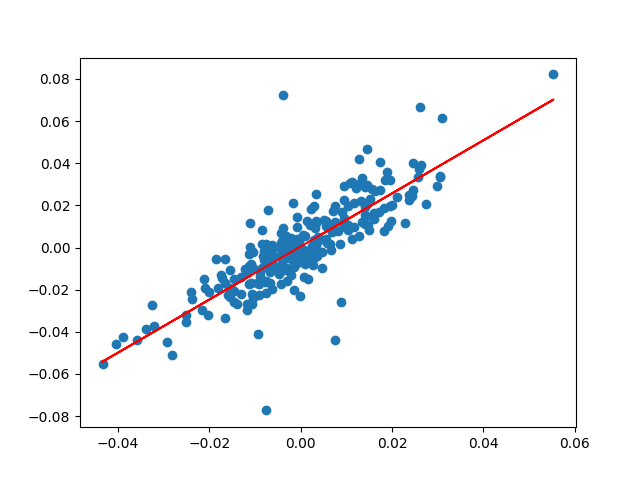
print(a.round(5), b.round(5)) # today, this gives me 0.00061 1.20539
A b of 1.2 means that MSFT is heavily dependent on market returns, but more volatile than the market.
This is a plot of the daily adjusted returns of MSFT and S&P 500,
together with the linear regression line:
Now, to use the CAPM model to predict the expected return of MSFT, we can use
# Compute the expected return of MSFT
expected_return = risk_free_rate + b * (sp500_returns.mean() - risk_free_rate) + a
Today, this gives me 0.00097 which annualised is (1 + 0.00045)^252 - 1 = 27%!
If we break down the terms in the expression above, it will be obvious that most of the contribution comes from alpha (~0.006).
Accounting just for the risk term, the annualised return we get is 9.5%. Let’s keep this number in mind.
DCF
The Discounted Cash Flow (DCF) model is a way to estimate the value of a stock given the expected future cash flows of the company.
To value a stock according to DCF, we project the future cash flows of the company and then discount them to the present. Microsoft has 7.411 billion outstanding shares, and its last reported net earnings are \$71.5 bn. We computed that the risk premium of MSFT is 9.5%.
Let’s assume that this is going to be the case for the next 10 years. We’ll also assume some growth: maybe we believe that Microsoft can grow at a rate of 12% for a few more years (5?), after which the company will grow at 9%, 8%, 7%… until it hits a terminal rate of 3.3% (the risk-free rate) on year 10.
These numbers are very important assumptions and growth rate estimates are not easy to come up with.
The future value of a present cashflow at a future time n is
CF(n) = CF(0) * (1 + g)^n
where CF(0) is the present value of the cash flow and g is the expected growth rate.
To discount this future value to the present, we use the discount rate k:
DCF(n) = CF(n) / (1 + k)^n
So each cash flow can be presently valued as
DCF(n) = CF(0) * (1 + g)^n / (1 + k)^n
The sum of all the cash flows is the value of the company (“enterprise value”):
EV = Sum(DCF(n)) for n in [1, \infty)
Let’s code this up.
def discounted_cashflow(cf, g, k, n):
    """ Present value of a future cashflow at time n """
    return cf * (1 + g)**n / (1 + k)**n

g = 0.12
g_terminal = 0.033
k = 0.095
cf = 71.5 # net income in bn
# up to year n = 5
value = 0
for n in range(1, 6):
    value += discounted_cashflow(cf, g, k, n)

# from year n = 6 to n = 10, the growth rate changes
rate_change = (g - g_terminal) / 4
for n in range(6, 10):
    g -= rate_change
    value += discounted_cashflow(cf, g, k, n)

# from year n = 10
for n in range(10, 500):
    delta = discounted_cashflow(cf, g, k, n)
    value += delta
    if delta < 0.01:
        break

value # 1,319.13
So the enterprise value according to our valuation model would be \$1,319.13 bn. To get our market cap estimate, we can subtract the total cash assets (\$100 bn) and subtract debt (\$60 bn) taken from Microsoft’s balance sheet. This results on a market cap of \$1,279 bn, or \$172 per share.
In theory, this would suggest that this stock, currently sitting at \$305, is massively overvalued. However, there are a few caveats to this model.
Firstly, it assumes a constant (or stepwise) growth rate and discount rate, which is not realistic. In fact, we saw above that Microsoft returns are highly correlated with the market. It also overlooks the elephant in the room: the big premium on microsoft stocks due to the opportunity with AI.
The importance of this exercise is that it gives a fundamentals-based estimate that we can forecast around. Do you think that AI will be a huge opportunity for Microsoft? Then that might justify the current price. Do you think that AI will be a flop? Then you might want to sell.